Affine Transformations

Introduction

My Linear Algebra education was pretty typical, I learned about eigenvalues, matrices, and transformations just well enough to pass exams, without really understanding why any of it mattered. That changed at my first job when I used it to transform LiDAR points across coordinate frames, finally seeing how these abstract concepts translate to real problems.

I thought I had a decent grasp on transformations after that. Then I tried rotating a bounding box around its center for a computer vision project, and it kept flying off to random parts of the image. Turns out I was missing something fundamental about how affine transformations actually work.

The Problem

Create a bounding box that contains a region of interest and apply an affine transformation to it.

What Are Affine Transformations and Why Do They Matter?

An Affine Transformation lets you scale, rotate, shear, and move points in space, all with a single compact matrix.

Before we begin, lets take a look into where Affine Transformations are used in real-world applications today:

• Image processing - for manipulating images and objects, tracking objects, etc.
• Augmented reality - for creating virtual simulated environments relative to a perspective
• Robotics - for tracking movements, object detection, mapping
• Gaming - usually used to move objects in space or around a screen

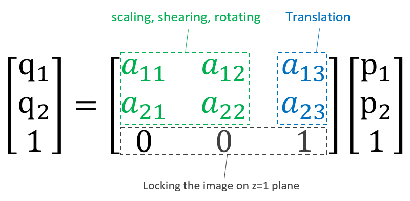
The Formula

An Affine Transformation is essentially a matrix of elements that serve as dials to a specific point. What these dials do is allow a user to change the geometry or shape or location of a specific point relative to an origin. For simplicity, this post will only cover 2D transformations but we can do this for 3D points as well.

How points get transformed using matrix multiplication in code:

/**
 * @brief Applies a 2D affine transformation to a point
 *
 * Transformation Matrix:
 * [x'] = [a b tx] [x]
 * [y']   [c d ty] [y]
 * [1 ]   [0 0  1] [1]
 *
 * Formula:
 * x' = ax + by + tx
 * y' = cx + dy + ty
 */
point transform_point(const point &p, double a, double b, double c, double d, double tx, double ty)
{
    double x_prime = a * p.x + b * p.y + tx;
    double y_prime = c * p.x + d * p.y + ty;
    // Round to int for point type
    return point{static_cast<int>(std::round(x_prime)), static_cast<int>(std::round(y_prime))};
}

Breaking down the transformation matrix components:

• a, d: Scaling (make objects bigger/smaller)
• Combination of a, b, c, d: Rotation (spin objects)
• b, c: Shearing (skew or slant)
• tx, ty: Translation (move or shift)

Bounding Boxes in Computer Vision

Bounding Boxes are rectangular regions that enclose objects of interest. They are often used in object tracking, region of interest selection, and object detection in computer vision.

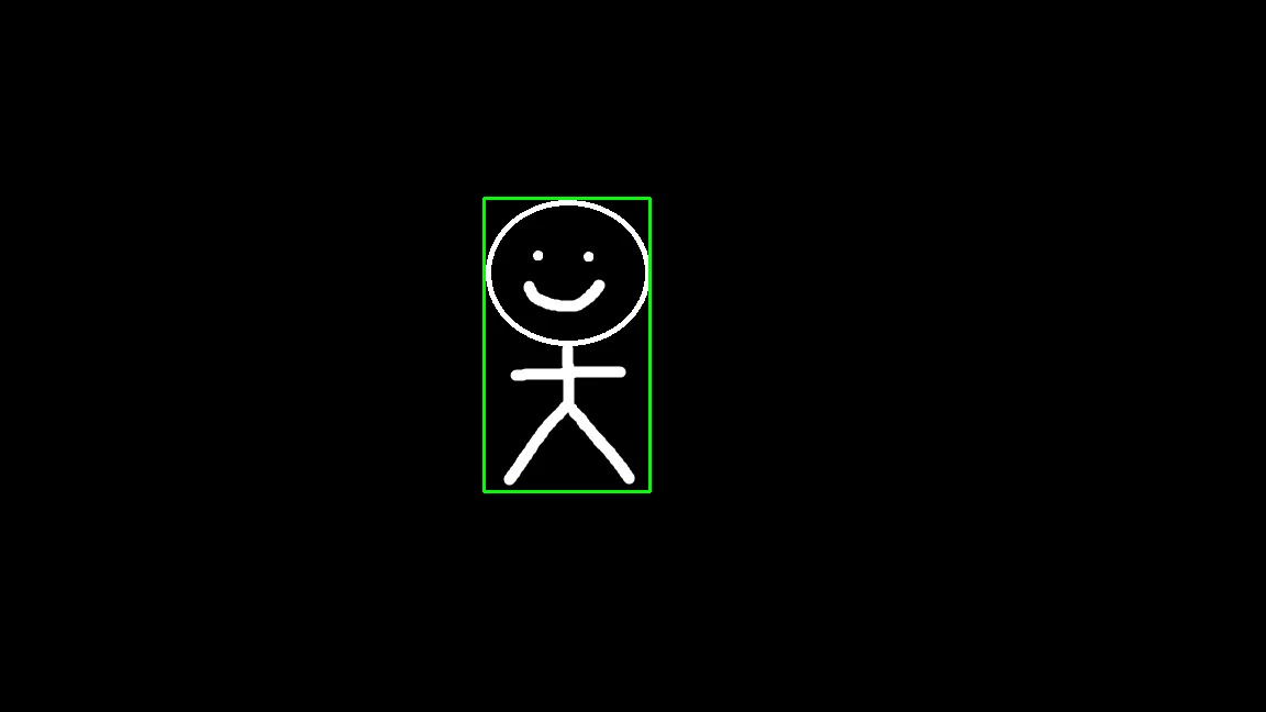
To demonstrate this example, I created this binary image using Paint of a simple character.

Next, we compute the bounding box of this character which produces a bounding box that looks like this:

How do bounding boxes relate to transformations?

When we transform an image, we need to transform the bounding boxes too. If we want to transform the region of interest, essentially we can transform the bounding box to get its new geometry or shape or for keeping track of where the object is after image manipulation.

Visualizing the Transformations

What better way to view the transformations than to visualize them? To do this, I will transform the corner points of the bounding box in order to get the transformed bounding box and where it would be if we were to transform the object.

To do this, we create OpenCV utility functions for drawing the updated bounding boxes on the original image.

Initial Results: The Naive Approach

I started by applying transformations to the bounding box edges and trying to draw them as rectangles. Translation and scaling worked beautifully 🙂

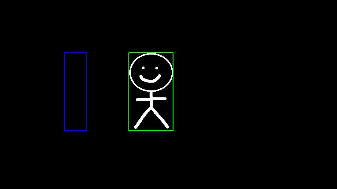
Translation - The bounding box shifted(translated) exactly as expected:

Scaling - The bounding box compressed(scaled) along the X-axis as intended:

However, when I tried rotation and shearing , something was clearly wrong. The visualizations didn’t show the expected rotated or sheared shapes at all!

The Issue: Axis-Aligned Bounding Boxes

The problem I ran into:

• The bounding boxes always stayed axis-aligned (their edges are parallel to the image edges).
• So when I tried to apply rotation or shear, nothing seemed to visually happen, even though the math said it did.

A normal bounding box can’t represent rotated or sheared shapes. The way that I was trying to visualize the transformation was wrong. It’s just a rectangle aligned to the axes, so any rotation or skewing gets “absorbed” and looks unchanged.

The fix: instead of redrawing the bounding box, I needed to draw a polygon connecting the transformed corner points. That way, I could actually see the rotation and shear as non-axis-aligned shapes.

Better Results… Mostly

After switching to polygons, things started looking a lot better.

Shearing - worked perfectly, I got a nice parallelogram just as expected in the x-direction.

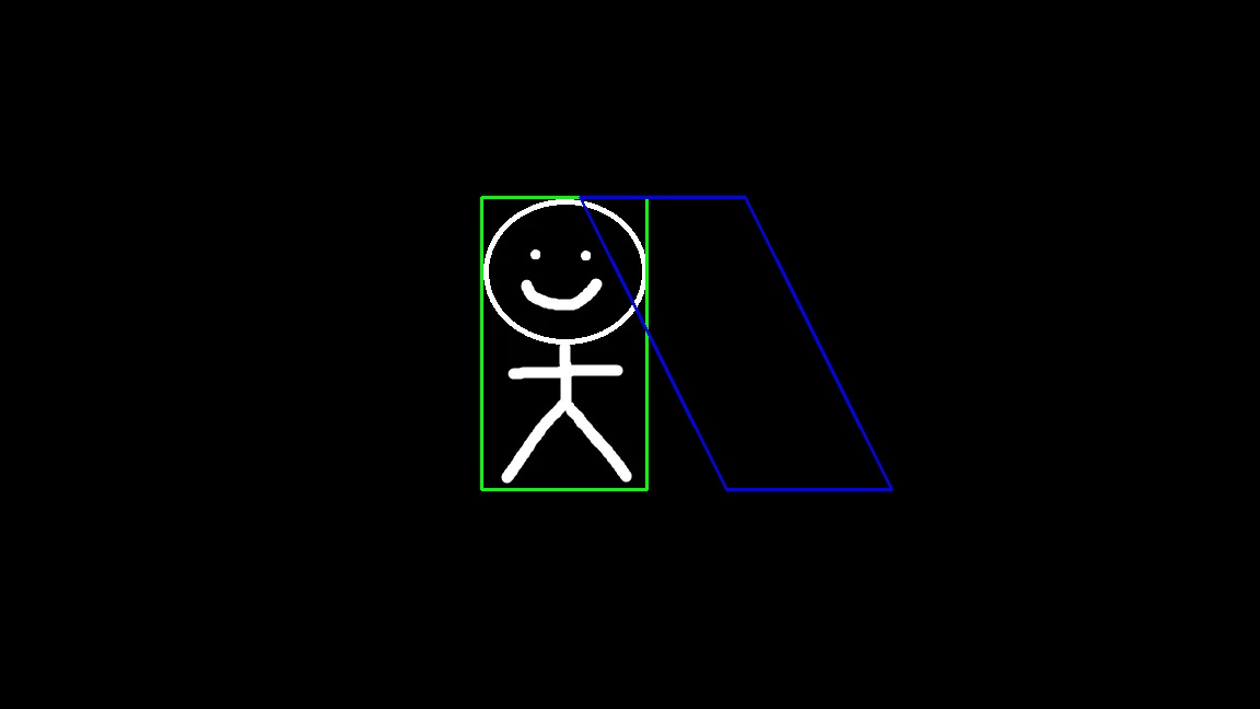
Rotation - was still way off.

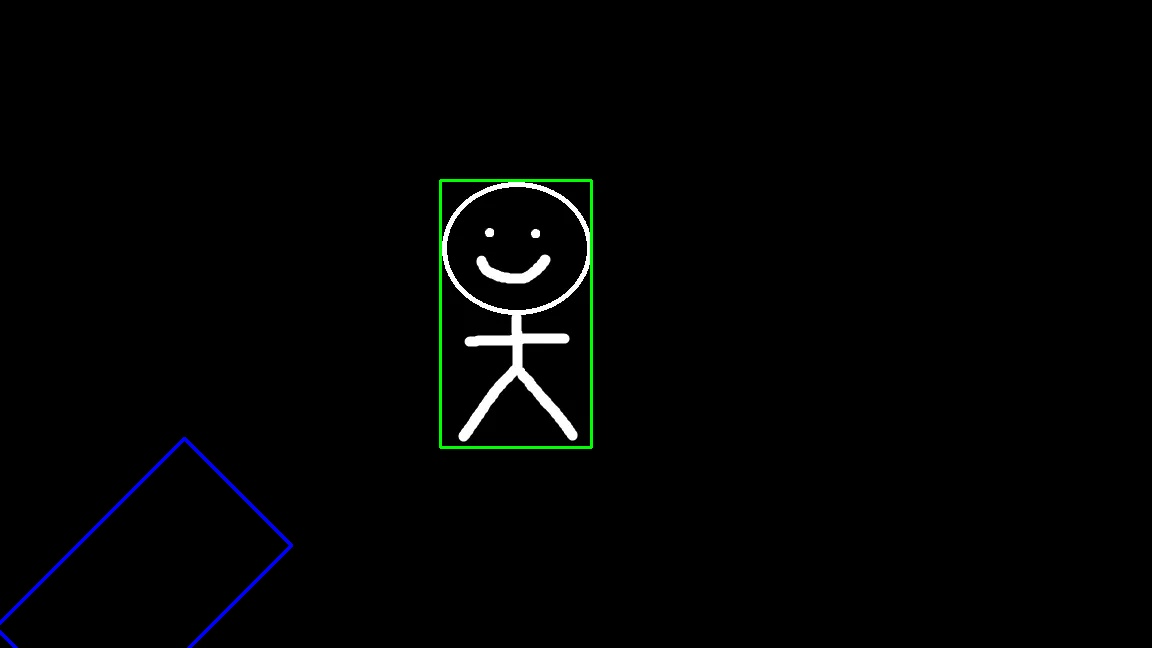
The box did rotate, but not around the character. It flew off to some random part of the image. Clearly, the math was doing something, just not what I was expecting.

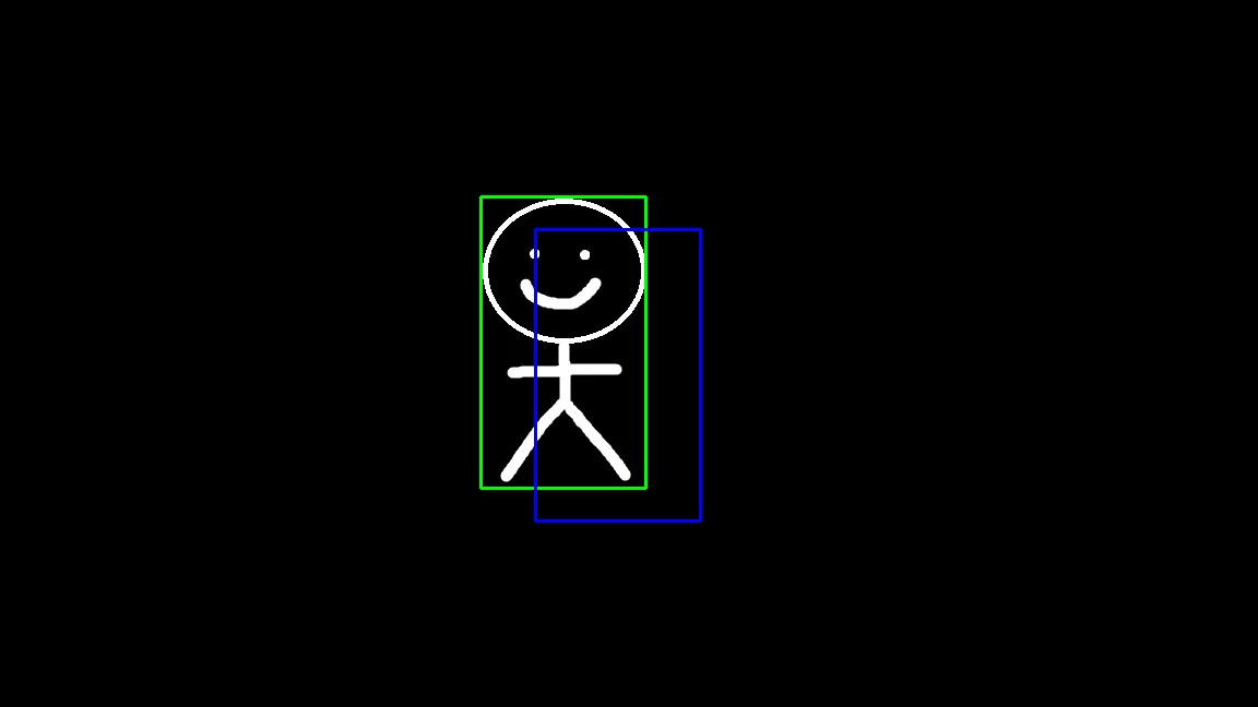
The Breakthrough 🤯

After some head scratching and research, I discovered a critical insight:

Affine transformations happen relative to the origin at (0, 0) - the top-left corner of the image!

So when you rotate something that’s far from the origin, its entire coordinate frame swings around a big circle centered at (0,0).

Why Did Rotation Look So Wrong?

What was really happening:

• My stick figure wasn’t near the origin, it is somewhere in the middle of the image.
• When I applied rotation, it didn’t spin around its own center, it spun around the image’s top-left corner.
• The farther an object is from that origin, the bigger the arc it travels.
• Result: The bounding box ended up way off from where I expected!

Why Did Other Transformations Look “Okay”?

Other transformations (like translation, scaling, or shear) technically happen relative to the origin too, but their effects are less dramatic:

• Translation - just moves everything by a fixed offset, so it behaves predictably.
• Scaling and shear - change shape and size but don’t create a huge circular movement like rotation does.
• Rotation - swings points along an arc, so displacement becomes much more dramatic when the object is far from (0, 0).

The Solution: Transform the Coordinate System

This realization led to the proper solution:

1. Translate the object so its center is at the origin
2. Rotate around the now-centered object
3. Translate back to the original position

Here’s the updated code that implements center-based rotation:

TEST(SimpleGuy, RotationCenter)
{
    cv::Mat image = cv::imread("simple_guy.jpg", cv::IMREAD_GRAYSCALE);
    bounding_box_edges original_edges = find_minimum_bounding_box(image);

    cv::Mat result;
    cv::cvtColor(image, result, cv::COLOR_GRAY2BGR);

    // Compute center point of the bounding box
    rectangle rect = utility::convert_edges_to_rectangle(original_edges);
    int center_x = std::round(rect.origin.x + rect.width / 2.0);
    int center_y = std::round(rect.origin.y + rect.height / 2.0);

    // Rotation (45 degrees)
    double angle = M_PI / 4.0;
    double cos_a = std::cos(angle);
    double sin_a = std::sin(angle);

    // Get original corners, doesn't perform anything because this is the identity matrix
    // We only use to grab the corner points of bounding box
    std::array<point, 4> corners = transform_bounding_box_corners(original_edges,
                                                                  1, 0, 0, 1,
                                                                  0, 0);

    // Rotation matrix but with adjusted points
    auto rotate_around_center = [&](const point &p)
    {
        // Translate the point so the desired rotation center moves to the origin
        point translated_point = transform_point(p,
                                                 1, 0, 0, 1,
                                                 -center_x, -center_y);
        // Rotate around the origin
        point rotated_point = transform_point(translated_point,
                                              cos_a, -sin_a, sin_a, cos_a,
                                              0.0, 0.0);
        // Translate back to restore the original position
        return transform_point(rotated_point,
                               1, 0, 0, 1,
                               center_x, center_y);
    };

    // Apply rotation around center
    std::array<point, 4> rotated_corners;
    for (size_t i = 0; i < 4; ++i)
        rotated_corners[i] = rotate_around_center(corners[i]);

    // Draw original (green)
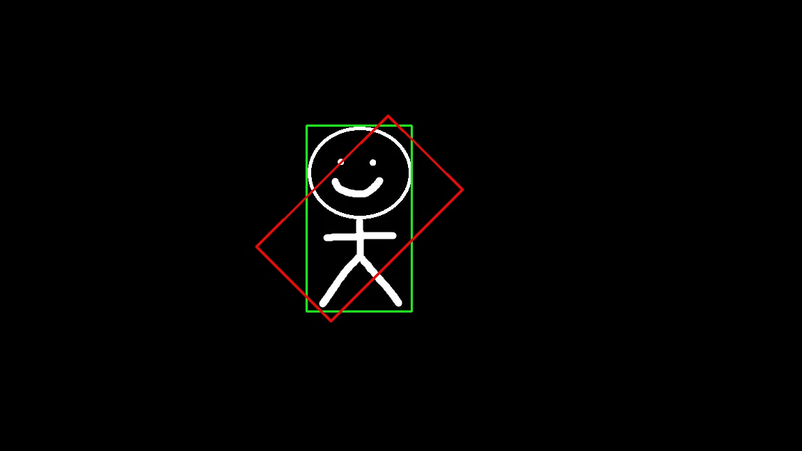
    utility::draw_rectangle(result, original_edges.to_rectangle(), cv::Scalar(0, 255, 0));

    // Draw rotated (red)
    utility::draw_polygon_from_corners(result, rotated_corners, cv::Scalar(0, 0, 255), 2);

    cv::imwrite("simple_guy_rotated_center.jpg", result);
}

The result : Perfect rotation around the center!

Conclusion

This was a fun weekend crash course on understanding affine transformations and visualizing them. I learned:

• The importance of understanding coordinate systems and reference points and that the origin of the image actually matters.
• The value of visualization in debugging mathematical operations
  • seeing the transformations helped me understand what was going wrong
• Why different transformations have different visual impacts
  • distance from the origin determines how dramatic the effect appears

These fundamentals contribute to many computer vision applications and I’m only scratching the surface of what’s possible. In the future, I’m excited to explore more OpenCV capabilities and 3D transformations.

Overall, documenting this has helped solidify my understanding and further expands my appreciation for Linear Algebra in the real world.