Exponential Moving Average

Introduction: Smoothing Noisy Sensor Data

When working with sensors, one of the first challenges you’ll run into is noise. Even a steady signal can look like it’s bouncing around, making it hard to get stable readings or build reliable control systems.

A common solution is to apply some form of smoothing to the data before using it. In this post, I’ll walk through a simple but powerful technique called the Exponential Moving Average (EMA) , show how I implemented it in C++, and demonstrate how adjusting its parameters changes how quickly (or slowly) your readings settle into a smooth output.

Why Smoothing Data is Useful?

Smoothing or some type of filtering on data is useful for easier visualization of the data and more reliable decision making . The focus on this post will be on the Exponential Moving Average (EMA) as a simple and effective method to perform these adjustments on my sensor’s data.

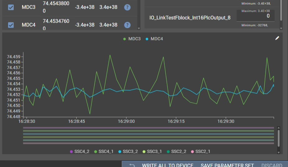
In the image above, the green line represents the raw real-time sensor output data and the turquoise line represents that data after an EMA filtering.

Notice how the turquoise line is much more stable and smooths out the noise to provide a clean steady representation of the raw sensor data.

What is an Exponential Moving Average?

An Exponential Moving Average (EMA) is a way to smooth out data by giving more weight to recent values while still considering older ones.

Example: Average Temperature Imagine you’re tracking the temperature each day to get a sense of the “average” temperature lately. With a regular average, each day counts equally. But with an EMA, yesterday’s temperature matters more than the day before, which matters more than the day before that, and so on.

The influence of older temperatures fades exponentially - hence the name.

The EMA Formula

The Exponential Moving Average formula is quite straightforward 😅:

EMA = (new_value × α) + (previous_EMA × (1 - α)) 

Where:

• α (alpha) is the smoothing factor
  • The smoothing factor α determines how much weight to give recent data.
  • A higher α (closer to 1) → the EMA more reactive to recent changes
  • a lower α (closer to 0) → the EMA is smoother and less reactive
• new_value: is the current data point
• previous_EMA: is the previous day’s EMA value
• EMA : is the current EMA value for this current data point

Haha however, this formula is actually not that straightforward in my opinion. We can derive the above formula and create an easier to read and simplified version:

EMA = (new_value × α) + (previous_value × (1 - α))
EMA = (new_value × α) + (previous_value × 1) - (previous_value × α) 
EMA = (new_value × α) + previous_value - (previous_value × α)
EMA = (new_value × α) - (previous_value × α) + previous_value
EMA = α × (new_value - previous_EMA) + previous_EMA  🙂

and moving the variables around following the rules of mathematics we can rearrange this to be:

EMA = (new_value - previous_EMA) * α + previous_EMA  😀 

Ah! Much better! 👍

Example: Average Temperature In the Average Temperature example, the new_value would be our new current temperature point. And the previous_EMA would be our last calculated EMA value from yesterday’s temperature point.

But How Do We Calculate Alpha? 🤔

Aha! 💡 This is where we decide the parameters that will directly effect our EMA!

alpha can be calculated with the following equation:

alpha = (sampling_time / averaging_time) * multiplier

Where:

• sampling_time is your actual sensor sampling interval (could be in seconds , ms, etc.)
• averaging_time is the desired time constant (how long to reach ~63% of a step change and must be in same unit as the sampling time)
• multiplier adjusts convergence behavior (typically a constant value between 2-5 for faster settling)

Key advantages of EMA:

• gives more weight to recent values
• creates a smooth filtering on data points based on previous data
• reacts faster or slower to change depending on the user’s input parameters
• quick and easy to implement

Implementing EMA in C++

In C++ I created an ExponentialMovingAverage class to perform this data smoothing. Below is an example class that I wrote that takes the three parameters into it’s constructor which help us compute the alpha described above and allow us to update our latest EMA value.

  class ExponentialMovingAverage
  {
  public:

    ExponentialMovingAverage(float sampling_time, float averaging_time, float multiplier)
        : sampling_time(sampling_time),
          multiplier(multiplier),
          last_averaging_time(averaging_time),
          initialized(false)
    {
      compute_alpha(averaging_time);
    }

    // Return the updated ema value based on the new_value and 
    // new averaging time
    float update_ema(float new_value, float new_averaging_time)
    {
      // Recompute alpha only if new averaging time given
      if (new_averaging_time != last_averaging_time && averaging_time > sampling_time)
      {
        compute_alpha(new_averaging_time);
      }
      return update_ema(new_value);
    }

    // Return the updated ema value based on this new input value
    float update_ema(float new_value)
    {
      if (!initialized)
      {
        initialized = true;
        previous_value = new_value;
        return new_value;
      }

      float ema = (new_value - previous_value) * alpha + previous_value;
      previous_value = ema;
      return ema;
    }

  private:
    // Compute alpha based on the averaging time given
    void compute_alpha(float averaging_time)
    {
      alpha = (sampling_time / averaging_time) * multiplier;
      last_averaging_time = averaging_time;
    }

    float sampling_time;
    float multiplier;
    float alpha{1.0f};
    float last_averaging_time;
    float previous_value{0.0f};
    bool initialized;
  };

• We offer the user two public API calls to update the EMA that they can use:
  • update_ema(float new_value) : if they wish to never change the averaging time and simply update the ema value based off of the new data point value given.
  • update_ema(float new_value, float new_averaging_time) : if they wish to change the averaging time and compute a new alpha based off of this new averaging time and update the ema value based off of the new data point value given. Giving flexibility to the user!

Recall: The alpha variable controls responsiveness (a number between 0 and 1). So the input averaging time effects our alpha directly.

• A smaller averaging time → faster response
• A larger averaging time → smoother but slower response

Practical Usage Example

Now let’s see how we’d use this class in practice. First, we’d initialize our Temperature EMA with the following input parameters to compute alpha based on our requirements.

Example: Average Temperature Let’s say we were sampling temperature at a rate of 20ms and wanting the temperature to average out to its new value at a rate of 2seconds, with a convergence multiplier constant of 5, we’d do:

constexpr float TEMPERATURE_SAMPLING_TIME_S{0.02F}; // 20 ms
constexpr float TEMPERATURE_AVERAGING_TIME_S{2.0f};
constexpr float EMA_CONVERGENCE_MULTIPLIER{5.0f};
ExponentialMovingAverage ema{TEMPERATURE_SAMPLING_TIME_S, TEMPERATURE_AVERAGING_TIME_S,
                                    EMA_CONVERGENCE_MULTIPLIER};

And updating the EMA we’d provide a simple call in our runtime code like this:

  void update_temperature()
  {
    float current_temp{sensor.get_current_temp()};
    float temperature_deg_C = ema.update_ema(current_temp);
    other_object.set_temperature(temperature_deg_C);
  }

Lets also remember that the ExponentialMovingAverage class offers flexibility — averaging time can be changed dynamically if needed! If the user would want to change the ema responsiveness they could update the averaging_time

void update_temperature()
{
  float current_temp{sensor.get_current_temp()};
  float input_averaging_time{user.get_input_avg_time()};
  float temperature_deg_C = ema.update_ema(current_temp, input_averaging_time);
  other_object.set_temperature(temperature_deg_C);
}

Comparison: Different Averaging Times 📈

When we apply EMA in practice, it doesn’t just smooth out noise — it also controls how fast the system reacts to changes . This balance depends entirely on the averaging time you choose.

A small averaging time makes the EMA quick to follow sudden changes, but with less smoothing. A large averaging time makes the signal very stable, but slower to catch up when the input shifts.

• Small averaging time → fast response, less smoothing
• Large averaging time → slow response, strong smoothing

The graphs below show this trade-off in action.

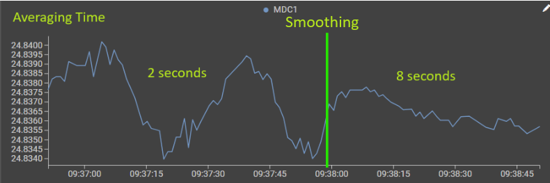
The Left side (2-second averaging time):

• Reacts quickly to sensor changes
• More responsive but potentially noisier
• Sharp transitions when the underlying data changes
• Good for applications where you need fast response to real changes

Right side (8-second averaging time):

• Much smoother and more stable
• Slower to respond but filters out short-term fluctuations
• Gradual transitions that reduce noise and sudden spikes
• Better for applications where stability is more important than immediate response

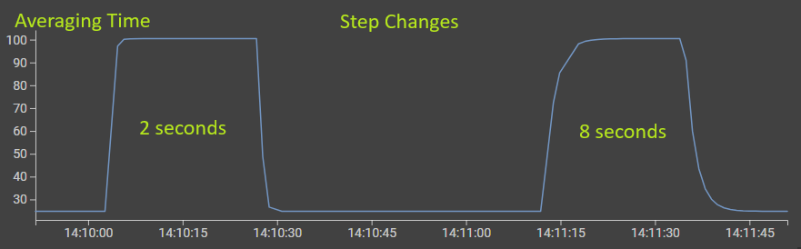
2-second averaging time (left):

• Sharp, quick step response - reaches the new value rapidly
• Minimal transition time when new data arrives
• Almost immediate adaptation to changes

8-second averaging time (right):

• Gradual, smooth step response - takes much longer to reach the new value
• Extended transition period with a curved approach
• Much more gradual adaptation to the same input change
• The signal takes much longer to “catch up” to the new value.

Trade-offs: Responsiveness vs. Stability

In practice, tuning EMA is always about finding the sweet spot between responsiveness and stability . The “right” averaging time depends on your application — whether you need a system that reacts quickly to change or a steady signal.

Conclusion: Two Tools In One 🛠️

The Exponential Moving Average is lightweight, tunable, and effective for real-time applications — whether you’re working with sensors or tracking market prices.

The beauty of EMA is that it’s two tools in one:

1. A noise filter that stabilizes jittery signals.
2. A responsiveness dial that controls how quickly your system adapts to change.

By tuning the averaging time, you get to choose whether your system should prioritize speed or stability. For many real-world applications, choosing the right balance between the two is exactly what’s needed.

If you’re experimenting with sensors in your own projects, play around with different averaging times and watch how the filter behaves — you’ll quickly see how powerful a few lines of code can be.

Cheers fam✌🏻,

Eduardo