Understanding Simd Intrinsics
Speeding up computation through CPU level vectorization

Introduction
I recently learned about intrinsics and thought it’d be a good idea to document my understanding of them by explaining what they are, how they work under the hood, and how we can utilize them to have faster and more performative code.
When Performance Matters
Real time applications often demand intense numerical processing on large amounts of data. When we rely on basic scalar calculations (operating on one data value at a time) we create latency that limits our application’s performance. This performance slow down can be critical if our application requires real-time responsiveness.
Modern CPUs offer a solution! SIMD (Single Instruction, Multiple Data) intrinsics. By leveraging SIMD intrinsics, we can achieve significant speedups in the processing of our data utilizing vector storage on the CPU.
What Are Intrinsics❓
Intrinsics are special functions that allow us to perform the same operation on multiple pieces of data simultaneously using a single CPU instruction. Unlike regular C++ functions that the compiler translates into multiple assembly instructions, intrinsics give us direct access to low-level CPU operations.
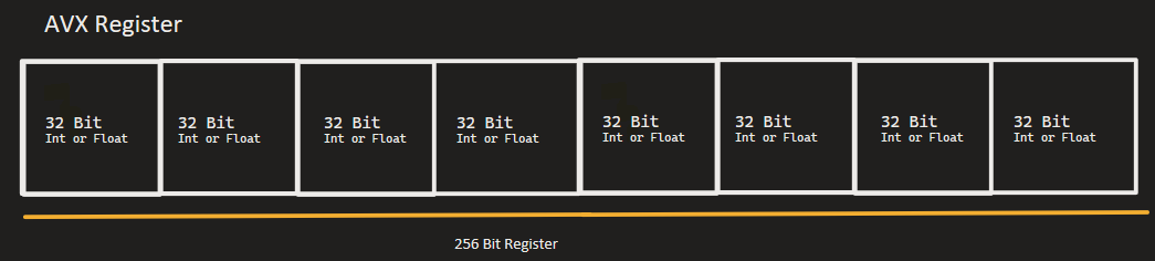
SIMD intrinsics specifically utilize vector registers in the CPU, using special hardware designed to hold and operate on multiple values at once. These registers come in different sizes depending on the instruction set:
- SSE/SSE2 (Stream Extension): 128-bit registers (4 × 32-bit integers or floats)
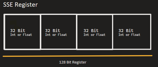
- AVX/AVX2 (Advanced Vector Extension): 256-bit registers (8 × 32-bit integers or floats)
How The CPU Stores Data
To understand why SIMD is powerful, we need to understand how the CPU organizes data.
Regular variables are stored in memory and loaded into general purpose registers one at a time like this:
1
2
3
int a = 10;  // Stored in a 32-bit register
int b = 20;  // Stored in another 32-bit register
int c = a + b;  // One add instruction
SIMD registers on the other hand, can pack multiple values together. If we take a look at the SSE instruction set (for simplicity), the vector register can look like this:
1
2
3
4
5
6
Memory:     [10] [20] [30] [40]  (4 separate 32-bit integers)
                    ↓
            Loaded into a 128-bit register
                    ↓
Register:   [10 | 20 | 30 | 40]  (all 4 values in one 128-bit register)
When we perform an operation on a SIMD register, it applies to all packed values simultaneously.
Example: Array Summation Using SSE Intrinsics
Let’s implement a simple function that adds two arrays of four 32-bit integers using SSE intrinsics:
1
2
3
4
5
6
7
8
9
10
11
12
13
14
15
16
17
18
19
20
21
#include <immintrin.h> // API for accessing SIMD SSE intrinsic functions
#include <array>

/**
 * @brief Sums two arrays of 4 integers using SSE intrinsics
 */
std::array<int, 4> sum_integer_array_intrinsics(const int *a, const int *b)
{
    // Load 128 bits (4 integers) from memory into SSE registers
    __m128i vector_one = _mm_loadu_si128(reinterpret_cast<const __m128i *>(a));
    __m128i vector_two = _mm_loadu_si128(reinterpret_cast<const __m128i *>(b));

    // Perform element-wise addition in a single instruction
    __m128i vector_result = _mm_add_epi32(vector_one, vector_two);

    // Store the result into an array to return to the user
    std::array<int, 4> result{};
    _mm_storeu_si128(reinterpret_cast<__m128i *>(result.data()), vector_result);
    return result;
}
Breaking Down the Intrinsic Functions
_mm_loadu_si128 - Loads 128 bits of data from memo
_mm_add_epi32 - Adds packed 32-bit integers in one CPU instruction
- Performs 4 additions simultaneously:
[a0+b0, a1+b1, a2+b2, a3+b3]
_mm_storeu_si128 - Stores 128 bits back to memory
- Stores into the result C++ array
Visual Representation
1
2
3
4
5
6
7
8
9
10
11
12
13
14
15
16
17
        a: [10] [20] [30] [40]
              ↓    ↓    ↓    ↓
           _mm_loadu_si128
              ↓    ↓    ↓    ↓
vector_one: [10 | 20 | 30 | 40]  (packed in 128-bit register)

        b:  [1]  [2]  [3]  [4]
              ↓    ↓    ↓    ↓
           _mm_loadu_si128
              ↓    ↓    ↓    ↓
vector_two: [1  | 2  | 3  | 4]   (packed in 128-bit register)

              ↓    ↓    ↓    ↓
        _mm_add_epi32 (ONE instruction)
              ↓    ↓    ↓    ↓
result:     [11 | 22 | 33 | 44]  (4 additions in parallel)
Comparing Scalar vs SIMD
For comparison, here’s the scalar (non-SIMD) version of the above code:
1
2
3
4
5
6
7
8
9
10
std::array<int, 4> sum_integer_array_scalar(const int *a, const int *b)
{
    std::array<int, 4> result{};
    for (int i = 0; i < 4; i++)
    {
        result[i] = a[i] + b[i];  // 4 separate add instructions
    }
    return result;
}
Performance Characteristics
For this small example (only 4 elements), the performance difference is negligible due to only dealing with a small number of elements:
- SIMD version: load → add → store (but handles 4 values at once)
- Scalar version: 4 individual loads, adds, and stores
However, SIMD’s advantage becomes dramatic with larger arrays.
For example: Say we needed to perform an operation on a 1920×1080 image (2,073,600 pixels), we’d see significant speedup:
- Scalar version: 2,073,600 separate operations
- SIMD (SSE): 2,073,600 /4 = 518,400 operations (4× speedup)
- SIMD (AVX): 2,073,600 /8 = 259,200 operations (8× speedup)
This is a huge upgrade in performance and something we can now tell modern compilers to do for us without calling these intrinsic functions manually ourselves. This method of allowing the compiler perform intrinsics for us is referred to as “Auto Vectorization”.
Auto-Vectorization: The Compiler Does It For You 👍🏻
Modern compilers can automatically generate SIMD instructions from regular code when you enable optimization flags. To test this, we can open up godbolt and write some code that essentially does some basic computation for us similar to what we’re doing above with the scalar example.
1
2
3
4
5
6
7
8
9
10
11
12
13
14
15
16
#include <array>

std::array<int, 4> sum_arrays(const int* a, const int* b) {
    std::array<int, 4> result;
    for (int i = 0; i < 4; i++)
        result[i] = a[i] + b[i];
    return result;
}

int main()
{

    int one[4] = {10,20,30,40};
    int two[4] = {1,2,3,4};
    auto sum_array = sum_arrays(one, two);
}
With no optimization flags, we see this monster of an assembly output:
1
2
3
4
5
6
7
8
9
10
11
12
13
14
15
16
17
18
19
20
21
22
23
24
25
26
27
28
29
30
31
32
33
34
35
36
37
38
39
40
41
42
43
44
45
46
47
48
49
50
51
52
53
54
55
56
57
58
59
60
61
sum_arrays(int const*, int const*):
        push    rbp
        mov     rbp, rsp
        push    rbx
        sub     rsp, 56
        mov     QWORD PTR [rbp-56], rdi
        mov     QWORD PTR [rbp-64], rsi
        mov     DWORD PTR [rbp-20], 0
        jmp     .L2
.L3:
        mov     eax, DWORD PTR [rbp-20]
        cdqe
        lea     rdx, [0+rax*4]
        mov     rax, QWORD PTR [rbp-56]
        add     rax, rdx
        mov     edx, DWORD PTR [rax]
        mov     eax, DWORD PTR [rbp-20]
        cdqe
        lea     rcx, [0+rax*4]
        mov     rax, QWORD PTR [rbp-64]
        add     rax, rcx
        mov     eax, DWORD PTR [rax]
        lea     ebx, [rdx+rax]
        mov     eax, DWORD PTR [rbp-20]
        movsx   rdx, eax
        lea     rax, [rbp-48]
        mov     rsi, rdx
        mov     rdi, rax
        call    std::array<int, 4ul>::operator[](unsigned long)
        mov     DWORD PTR [rax], ebx
        add     DWORD PTR [rbp-20], 1
.L2:
        cmp     DWORD PTR [rbp-20], 3
        jle     .L3
        mov     rax, QWORD PTR [rbp-48]
        mov     rdx, QWORD PTR [rbp-40]
        mov     rbx, QWORD PTR [rbp-8]
        leave
        ret
main:
        push    rbp
        mov     rbp, rsp
        sub     rsp, 48
        mov     DWORD PTR [rbp-16], 10
        mov     DWORD PTR [rbp-12], 20
        mov     DWORD PTR [rbp-8], 30
        mov     DWORD PTR [rbp-4], 40
        mov     DWORD PTR [rbp-32], 1
        mov     DWORD PTR [rbp-28], 2
        mov     DWORD PTR [rbp-24], 3
        mov     DWORD PTR [rbp-20], 4
        lea     rdx, [rbp-32]
        lea     rax, [rbp-16]
        mov     rsi, rdx
        mov     rdi, rax
        call    sum_arrays(int const*, int const*)
        mov     QWORD PTR [rbp-48], rax
        mov     QWORD PTR [rbp-40], rdx
        mov     eax, 0
        leave
        ret
The Beauty Of Optimization Flags
By changing the optimization level through a compiler flag, lets say -O1 (basic optimization) we see the following assembly produced:
1
2
3
4
5
6
7
8
9
10
11
12
13
14
15
sum_arrays(int const*, int const*):
        mov     eax, 0
.L2:
        mov     edx, DWORD PTR [rsi+rax]
        add     edx, DWORD PTR [rdi+rax]
        mov     DWORD PTR [rsp-24+rax], edx
        add     rax, 4
        cmp     rax, 16
        jne     .L2
        mov     rax, QWORD PTR [rsp-24]
        mov     rdx, QWORD PTR [rsp-16]
        ret
main:
        mov     eax, 0
        ret
Much better! This makes me see how truly valuable godbolt is as a resource. To be able to see your compiled code in assembly and see what is going on underneath the hood with different optimization flags is eye opening. This resource would’ve been extremely beneficial for me in introductory programming classes!
However, it seems we can do even better than this by upping the optimization flag to -O3 (most aggressive optimization) which enables the best possible performance.
With the -O3 compile flag set, the compiler will often emit the same SIMD instructions as our manual intrinsics version. Here is a godbolt example on the above code to verify the assembly updates with the aggressive optimization:
1
2
3
4
5
6
7
8
9
10
11
sum_arrays(int const*, int const*):
        movdqu  xmm1, XMMWORD PTR [rsi]
        movdqu  xmm0, XMMWORD PTR [rdi]
        paddd   xmm1, xmm0
        movaps  XMMWORD PTR [rsp-24], xmm1
        mov     rax, QWORD PTR [rsp-24]
        mov     rdx, QWORD PTR [rsp-16]
        ret
main:
        xor     eax, eax
        ret
What Happens When Data Is Not A Multiple Of The Vector Register?
Let’s say we have 102 integers and we’re using the SSE instruction set, which can process 4 integers per vector register. The first 100 values (25 groups of 4) are handled with SIMD instructions, and the remaining 2 values are processed normally in scalar mode.
This small leftover is completely fine — we would still get almost the full SIMD performance benefit.
When SIMD Isn’t the Answer
SIMD works best when:
- You have large amounts of data (hundreds to millions of elements)
- Operations are uniform (same operation applied to each of the elements)
- Data is contiguous in memory (arrays/vector)
- There’s minimal branching or complex logic
SIMD struggles with:
- Small datasets (overhead exceeds benefit)
- Scattered data (operations are expensive)
- Different control flow (different operations per element)
Practical Applications
SIMD intrinsics are widely used in:
- Image Processing: Applying filters, color corrections, or transformations to millions of pixels.
- Point Cloud Processing: Transforming or filtering millions of 3D points in robotics and autonomous vehicles.
- Audio Processing: Applying effects or mixing to audio samples in real-time.
- Machine Learning: Matrix operations and neural network computations.
- Cryptography: Hash functions and encryption algorithms.
Conclusion
SIMD intrinsics give us direct access to the CPU’s parallel capabilities, leading to huge performance boosts for data-heavy code. Instead of doing one operation at a time, SIMD lets us pack multiple values into a single register and operate on them simultaneously. Intrinsic functions are fundamental to modern high performance computing. For applications processing large amounts of data, leveraging SIMD can mean the difference between slow performance and real-time responsiveness.